kriging
Ordinary Kriging
Poisson Kriging-Area to Area
Poisson Kriging-Area to Point
These are the three types inside https://github.com/szymon-datalions/pyinterpolate
I also wan to show how to apply them to satellite image as an practice for APTRK
General Introduction
Reference: https://www.youtube.com/watch?v=J-IB4_QL7Oc
Problem Setup

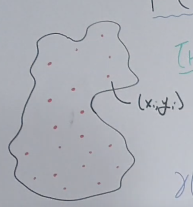
Here we have a island and we take some measurement for some red points. Each point include two attributes. xi is the location and yi is the thing we are interested in, like elevation.
Now we want to get the elevation in some other point that we did not explicitly collect data. For example in this black dot.

So we just could use the data we have to predict the elevation of black dot. There are five closest red dots to this unknown dot. We are gonna to use these five dots to predict the unknown dots. $$ y_{new}=w^Ty+\epsilon_{new}\\ =w_1y_1+w_2y_2+...+w_5y_5+\epsilon_{new} $$ This is a linear combination weight of neighbor dots. This is the kirging model. So the important thing is to know the w .
Variogram
A general idea is that the closer one should have higher weigh. But how do I formalize this idea in math? Here the things determines the weight is called the variogram. $$ \gamma(x_i,x_j)=\frac{1}{2}(y_i-y_j)^2 $$ This is the equation of variogram. (xi,xj) indicate the distance between two points. The distance is the input of γ function. And the output of γ function is half the difference of elevation. It should be increasing function since the smaller distance, the smaller difference.
So lets plot the graph between H, the distance (xi,xj) and the output of γ function.

This graph should reach the plateau as H increase. Because if the distance is two large, the difference should be almost the same, which indicate that the elevation belong to different group.
There are some terminology here. First is the nugget. The nugget is the intercept that our graph begin. It should be not equal to zero. Because the variogram is a fit line and maybe we have a lot of closed dot with different elevation. But it shoul be small.
Second one is the sill. Sill is the silling of a variogram. And the he range is the H value of sill.
Solving model
So we can get the weight from the variogram by solving a matrix equation.
Aw = b
Here A is the γ(xi,xj) and b is the γ(xnew,xi), w is the vector from w1 tow5
So I can just take a inverse to get the w.
Several Assumpution
- Stationarity: In every small part of island, the change speed of elevation should be almost the same.
- Constant variogram. In every small part of the island, the variogram shoul be almost the same.
Pros and Cons
Pros: we can estimate the error
Cons: For every new point, we need to solve different equation matrix.
Ordinary Kriging
Refference: Olea R A. Geostatistics for engineers and earth scientists[M]. Springer Science & Business Media, 2012.
The kriging model we describe before is the ordinary kriging. Kriging covers a range of least-squares methods of spatial prediction.
- Ordinary kriging of a single variable, as described in Section 8.2, is the most robust method and the one most used.
- Simple kriging (Section 8.9) is rather little used as it stands because we usually do not know the mean. It finds application in other forms such as indicator and disjunctive kriging in which the data are transformed to have known means.
- Lognormal kriging (Section 8.10) is ordinary kriging of the logarithms of the measured values. It is used for strongly positively skewed data that approximate a lognormal distribution.
- Kriging with drift (Chapter 9), also known as universal kriging, recognizes both non-stationary deterministic and random components in a variable, estimates the trend in the former and the variogram of the latter, and recombines the two for prediction. This introduces residual maximum likelihood into the kriging procedure (see Section 9.2).
- Factorial kriging or kriging analysis (Chapter 9) is of particular value where the variation is nested, i.e. more than one scale of variation is present. Factorial kriging estimates the individual components of variation sepa- rately, but in a single analysis.
- Ordinary cokriging (Chapter 10) is the extension of ordinary kriging of a single variable to two or more variables. There must be some coregionaliza- tion among the variables for it to be profitable. It is particularly useful if some property that can be measured cheaply at many sites is spatially correlated with one or more others that are expensive to measure and are measured at many fewer sites. It enables us to estimate the more sparsely sampled property with more precision by cokriging using the spatial information from the more intensely measured one.
- Indicator kriging (see Chapter 11) is a non-linear, non-parametric form of kriging in which continuous variables are converted to binary ones (indicators). It is becoming popular because it can handle distribu- tions of almost any kind, and empirical cumulative distributions of estimates can be computed and thereby provide confidence limits on them. It can also accommodate ‘soft’ qualitative information to improve prediction.
- Disjunctive kriging (see Chapter 11) is also a non-linear method of kriging, but it is strictly parametric. It is valuable for decision-making because the probabilities of exceeding or not exceeding a predefined threshold are determined in addition to the kriged estimates.
- Probability kriging (not described further in this book) was proposed by Sullivan (1984) because indicator kriging does not take into account the proximity of a value to the threshold, but only its position. It uses the rank order for each value, zðxÞ, normalized to 1 as the secondary variable to estimate the indicator by cokriging. Chile`s and Delfiner (1999) and Goo- vaerts (1997) describe the method briefly.
- Bayesian kriging (not described further in this book) was introduced by Omre (1987) for situations in which there is some prior knowledge about the drift. It is intermediate between simple kriging, used when there is no drift, and universal kriging where there is known to be drift. The kriging equations are those of simple kriging, but with non-stationary covariances (Chile`s and Delfiner, 1999).
Here I just gonna to talk about the three kinds of kriging model. For further you can just find that textbook.
But before we talk more deeply about that two type. Lets write the former introduction more detailed.
THEORY OF ORDINARY KRIGING
The aim of kriging is to estimate the value of a random variable,Z, at one or more unsampled points or over larger blocks, from more or less sparse sample data on a given support, say z(x1), z(x2), ..., z(xN), at points x1, x2, ..., xN. The data may be distributed in one, two or three dimensions, though applications in the environmental sciences are usually two-dimensional.
Ordinary kriging is by far the most common type of kriging in practice,and for this reason we focus on its theory here. It is based on the assumption that we do not know the mean. If we consider punctual estimation first, then we estimate Z at a point x0by Ẑ(x0), with the same support as the data, by $$ \hat{Z}(\boldsymbol{x}_0)=\sum_{i=1}^{N}\lambda_i(\boldsymbol{x}_i), $$ where λi are the weights. To ensure that the estimate is unbiased the weights are made to sum to 1, $$ \sum_{i=1}^{N}\lambda_i=1 $$
Review about the unbiased, consistent, efficient estimator https://en.wikipedia.org/wiki/Consistent_estimator#Unbiased_but_not_consistent
and the expected error is E[Ẑ(x0)−Z(x0)] = 0.
The estimation variance is $$ var[\hat{Z}(\boldsymbol{x}_0)]=E[\{\hat{Z}(\boldsymbol{x}_0)-Z(\boldsymbol{x}_0)\}^2]\\ =2\sum_{i=1}^{N}\lambda_i\gamma(\boldsymbol{x}_i,\boldsymbol{x}_0)-\sum_{i=1}^{N}\sum_{i=1}^{N}\lambda_i\lambda_j\gamma(\boldsymbol{x}_i,\boldsymbol{x}_j) $$ where γ(xi,xj) is the semivariance of Z between the data pointsxi and xj, and γ(xi,x0) is the semivariance between the ith data point and the target point x0.
Semi variance:http://www.kgs.ku.edu/Tis/surf3/s3krig2.html
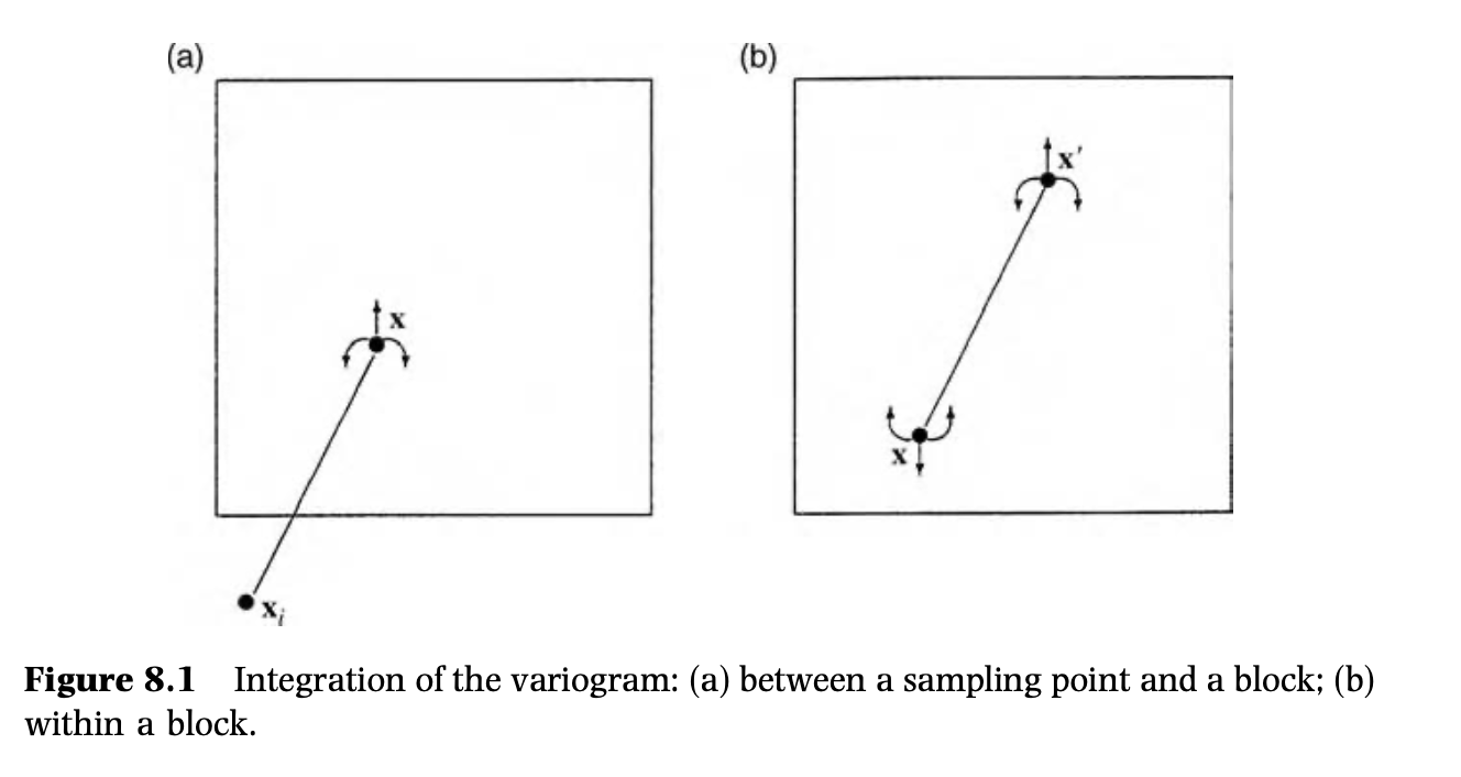
In the more general case we may wish to estimate Z in a block B, which may be a line, an area or a volume depending on whether it is in one, two or three spatial dimensions. The kriged estimate in B is still a simple weighted average of the data, $$ \hat{Z}(\boldsymbol{B})=\sum_{i=1}^{N}\lambda_iz(\boldsymbol{x}_i), $$ but with x0 of equation (3) replaced by B. Its variance is $$ var[\hat{Z}(\boldsymbol{B})]=E[\{\hat{Z}(\boldsymbol{B})-Z(\boldsymbol{B})\}^2]\\ =2\sum_{i=1}^{N}\lambda_i\gamma(\boldsymbol{x}_i,\boldsymbol{B})-\sum_{i=1}^{N}\sum_{i=1}^{N}\lambda_i\lambda_j\gamma(\boldsymbol{x}_i,\boldsymbol{x}_j)-\bar{\gamma}(B,B). $$ The quantity γ̄(xi,B) is the average semivariance between the ith sampling point and the block B and is the integral $$ $\bar\gamma(\boldsymbol{x}_i,B)$ =\frac{1}{B}\int_B\gamma(\boldsymbol{x}_i,\boldsymbol{x})d\boldsymbol{x}, $$ where γ(xi,x) denotes the semivariance between the sampling point xi and a point x describing the block.

The third term on the right-hand side of equation (7) is the double integral $$ \bar{\gamma}(B,B)=\frac{1}{|B^2|}\int_B\int_B\gamma(\boldsymbol{x},\boldsymbol{x^{\prime}})d\boldsymbol{x}d\boldsymbol{x^{\prime}} $$ where γ(x,x′) is the semivariance between two points x and x′ that sweep independently over B. It is the within-block variance. In punctual kriging γ̄(B,B)becomes γ̄(x0,x0) = 0, which is why equation (5) has two terms rather than three.
For each kriged estimate there is an associated kriging variance, which we can denote by σ2(x0) and σ2(B) for the point and block, respectively, and which are defined in equation(5) and equation(7).
The next step in kriging is to find the weights that minimize these variances, subject to the constraint that they sum to 1. We achieve this using the method of Lagrange multipliers.
Here I do not want to show how Lagrange multipliers works. Anyway this post is just a general introduction.
WEIGHTS
When the kriging equations are solved to obtain the weights, λi, in general the only large weights are those of the points near to the point or block to be kriged. The nearest four or five might contribute 80% of the total weight, and the next nearest ten almost all of the remainder. The weights also depend on the configuration of the sampling. We can summarize the factors affecting the weights as follows.
- Near points carry more weight than more distant ones. Their relative proportions depend on the positions of the sampling points and on the variogram: the larger is the nugget variance, the smaller are the weights of the points that are nearest to target point or block.
- The relative weights of points also depend on the block size: as the block size increases, the weights of the nearest points decrease and those of the more distant points increase , until the weights become nearly equal.
- Clustered points carry less weight individually than isolated ones at the same distance
- Data points can be screened by ones lying between them and the target
These effects are all intuitively desirable, and the first shows that kriging is local. They will become evident in the examples below. They also have practical implications. The most important for present purposes is that because only the nearest few data points to the target carry significant weight, matrix A in the kriging system need never be large and its inversion will be swift.
Covariance and Variogram
Before we step into the next one, we need to clarify some basic definition.
This part also comes from the previous textbook.