IOP inversion

This note is based on Lee 1998,1999,2002 and P. Werdell 2013

QAA

The reason for failure of QAA

After one year I found that I haven't finish the note. I will try to finish this.

But before that I think I found the reason for the failure of QAA

image-00021118142948938

Address: http://www.ioccg.org/groups/Software_OCA/QAA_v6_2014209.pdf

This is the whole process of QAA v6. Compared with the former one, the main update is in step2.

This is because in the first version, in the oligotrophic water, the \(a_{ph}\) is very low. Meanwhile the \(a_{CDOM}\) has a very influence in the \(a_{total}\) at 55xnm. So the \(a_{total}\) is mainly determined by \(a_w\). As a result, lee used an emprical relationship from \(r_{rs}\) to estimated \(a_{total}(55x)\). But in the coastal area, the \(a_{total}\) is dominated other constituents besides water, it make a lot of difference. It is also the reason that the update mainly happened in step2.

NIR base QAA

Some recent research use NIR wavelength for the step 2 as the non-water absorption at NIR is low.

Here is the 'A blended inherent optical property algorithm for global satellite ocean color observations'.

image-00021210194200562
image-00021210194014638

Another two is in Taihu.

image-00021210194504447
image-00021210194529712

QAA-750 is somewhat almost same with NIR-QAA, but QAA750-ap found that in Taihu, the ap750 sometime is still can't negletable.

We don't have ap763, I hope we can have that dataset later.

GIOP

This is another commly used Semi-analytical algorithm for IOP inversion.

This is the default algorithm of NASA IOP product

Introduction

  • SAA always differentiations only in the assumputions employed to define the eigenvectors and in the mathematical methods applied to calculate the eigenvalues
  • GIOP allows construction of different IOP models at runtime by selection from a wide assort-ment of published absorption and backscattering eigenvectors.

Method

Model Development

Lee et al 2002, Rrs to rrs \[ r_{rs}(\lambda,0^-)=\frac{R_{rs}(\lambda)}{0.52+1.7R_{rs}(\lambda)} \] rrs to IOP \[ r_{rs}(\lambda,0^-)=G_1(\lambda)u(\lambda)+G_2(\lambda)u(\lambda)^2 \]

\[ u(\lambda)=\frac{b_b{(\lambda)}}{a(\lambda)+b_b(\lambda)} \]

Common methods for estimating G?λ? include Gordon et al. [21], where G1 and G2 are spectrally fixed to 0.0949 and 0.0794 (see [7,23] for alternative coefficients), and the tabulated results ofMorel et al. [22], where G1 is estimated using solar and sensor geometries and an estimate of algal bio- mass and G2 is set to 0. GIOP supports all of these options.

IOP decomposition

each component can be expressed as the product of its concentration-specific absorption spectrum (eigenvector; a?) and its concentration or amplitude (eigenvalue; A): \[ a(\lambda)=a_w(\lambda)+\sum_{i=1}^{N}A_{ph}a_{ph}^{*}(\lambda)+\sum_{i=1}^{N}A_{d}a_{d}^{*}(\lambda)+\sum_{i=1}^{N}A_{g}a_{g}^{*}(\lambda) \] Both \(a_{d}^*(\lambda)\) and \(a_g^*(λ)\) are commonly expressed as \[ a_{d,g}^*(\lambda)=exp(-S_{d,g}\lambda) \] where Sd and Sg typically vary between 0.01 and 0.02 nm−1 in natural waters [24].

As the spectral shapes of NAP and CDOM absorption differ only in their exponential slopes, the two components are typically combined for satellite applications and Eq. (4) becomes

\[ a(\lambda)=a_w(\lambda)+\sum_{i=1}^{N}A_{ph}a_{ph}^{*}(\lambda)+\sum_{i=1}^{N}A_{dg}a_{dg}^{*}(\lambda) \] For total backscattering \[ b_b(\lambda)=b_{bw}({\lambda})+\sum_{i=1}^NB_{bp}b_{bp}(\lambda) \] Bbp provides the eigenvalue and a power function often represents the eigenvector: \[ b_{bp}^*(\lambda)=\lambda^{S_{bp}} \] where Sbp typically varies between −2 and 0 from small to large particles.

While commonly employed in the remote-sensing paradigm, we acknowledge the validity of the power function for b? bpλ remains debatable [25–27].

Using Rrsλ and eigenvectors as input, eigenvalues for absorption (A) and backscattering (B) can be estimated via linear or nonlinear least squares inversion of Eqs. (1)–(3).

Note that this model describes each component of absorption and back- scattering as a linear sum of subcomponents, presumably with unique spectral dependencies [sym- bolized by the summation over N in Eqs. (4), (6), and (7)]. In this way, the absorption characteristics for different phytoplankton populations and the scatter- ing characteristics of multiple size distributions of suspended particles can be represented, or Eq. (6) can be re-expanded to Eq. (4).

Model configuration

image-00021124160320671

Here explained the default configuration of GIOP.

Code

I think code is more visble for me

I skip the former part

1
2
3
4
5
6
7
8
9
10
11
12
13
14
15
16
17
18
19
20
21
22
23
24
25
26
27
28
29
30
31
32
33
34
35
36
37
38
39
40
41
42
43
44
45
46
47
48
49
50
51
52
53
54
55
56
57
58
59
60
61
62
63
64
65
66
67
68
69
70
71
72
73
74
75
76
77
78
79
80
81
82
83
84
85
86
87
88
89
90
91
92
93
94
95
96
97
98
99
100
101
102
103
104
105
106
107
108
109
110
111
112
113
114
115
116
117
118
119
120
121
122
123
124
125
126
127
128
'''
GIOP ocean color reflectance inversion model

P.J. Werdell and 18 co-authors, "Generalized ocean color
inversion model for retrieving marine inherent optical
properties," Appl. Opt. 52, 2019-2037 (2013).

GIOP is an ocean reflectance inversion model that
can be configured at run-time.

Requires equally-sized vectors of wavelength and Rrs
plus an estimate of chlorophyll; all other parameterizations
are controlled by the structure 'gopt', described below

Processing comments:
- defaults to GIOP-DC configuration
- currently requires 412, 443, and 547/555 nm to be present

Outputs are a vector of the magnitudes of the eigenvalues
for adg, bbp, and aph (x), plus modeled spectra of apg,
aph, adg, bbp, and Rrs

Rewritten in python via:
- C implementation (B. Franz, 2008) (https://oceancolor.gsfc.nasa.gov/docs/ocssw/giop_8c_source.html)
- Matlab implementation (J. Werdell, 2013)

Brandon Smith, NASA Goddard Space Flight Center, April 2018
'''

from MDN.Benchmarks.chl.OC.model import model3 as OC3
from MDN.Benchmarks.utils import get_required, optimize, loadtxt, to_rrs
from MDN.Benchmarks.meta import (
h0, h1, h2,
g0_Gordon as g0,
g1_Gordon as g1,
)

from scipy.interpolate import CubicSpline as Interpolate
from scipy.optimize import minimize
import numpy as np


# Define any optimizable parameters
@optimize([])
def model(Rrs, wavelengths, sensor, *args, independent=True, **kwargs):
'''
With independent=False, there is a dependency between sample
estimations - meaning the estimated parameters can vary wildly
depending on which samples are passed in.
'''
def bricaud(chl, wavelengths):
data = loadtxt('../IOP/bricaud_1998_aph.txt')
aphs = (data[:, 3] * chl ** (data[:, 4] - 1)).T
aphs *= 0.055 / aphs[data[:, 0] == 442]
return Interpolate(data[:, 0], aphs)(wavelengths).T

wavelengths = np.array(wavelengths)
required = [443, 555]
tol = kwargs.get('tol', 9) # allowable difference from the required wavelengths
Rrs = get_required(Rrs, wavelengths, required, tol)

aw = Interpolate(*loadtxt('../IOP/optics_coef.txt', ' ')[:, :2].T)(wavelengths)
bbw = 0.0038 * (400 / wavelengths) ** 4.32
chl = OC3(Rrs(None), wavelengths, sensor).flatten()[:, None]

rrs = get_required(to_rrs(Rrs(None)), wavelengths, required, tol)
eta = 2 * (1 - 1.2 * np.exp(-0.9 * rrs(443) / rrs(555)))
sdg = 0.018

aph = bricaud(chl, wavelengths)
bbp = (443 / wavelengths) ** eta
adg = np.exp(-sdg * (wavelengths - 443))
rrs = rrs(None)
## 前面的部分都是给这个优化设置初始值

assert (len(rrs) == len(chl) == len(bbp) == len(aph)), \
[rrs.shape, chl.shape, bbp.shape, aph.shape]

if independent:
aph = aph[:, None]
bbp = bbp[:, None]
rrs = rrs[:, None]

results = []
for _aph, _bbp, _rrs, _chl in zip(aph, bbp, rrs, chl):

# Function minimization
if True:
def cost_func(guess):
guess = np.array(guess).reshape((3, -1, 1))
atot = aw + _aph * guess[2] + adg * guess[0]
bbtot = bbw + _bbp * guess[1]
u = bbtot / (atot + bbtot)
rmod = g0 * u + g1 * u ** 2
cost = np.sum((_rrs - rmod) ** 2, 1) # Sum over bands

return cost.mean() # Average over samples
# 然后这里是通过一个优化的方式来得到最终确定的参数的,这个是cost function
init = [[0.01] * len(_chl), [0.001] * len(_chl), _chl]
res = minimize(cost_func, init, tol=1e-6, options={'maxiter': 1e3}, method='BFGS')
# res = minimize(cost_func, init, tol=1e-6, options={'maxiter':1e3}, method='SLSQP', bounds=[(0, 1e3)]*len(init))
# res = minimize(cost_func, init, tol=1e-10, options={'maxiter':1e5}, method='SLSQP')
x = np.array(res.x).reshape((3, -1, 1))
#求解的方式是Linear Matrix inversion
# Linear matrix inversion
else:
q = (-g0 + (g0 ** 2 + 4 * g1 * _rrs) ** 0.5) / (2 * g1)
b = (bbw * (1 - q) - aw * q).T
Z = np.vstack([np.atleast_2d(adg) * q, np.atleast_2d(_bbp) * (q - 1), np.atleast_2d(_aph) * q]).T
Q, R = np.linalg.qr(Z)
x = np.linalg.lstsq(R, np.linalg.lstsq(R.T, np.dot(Z.T, b))[0])[0]
r = b - np.dot(Z, x)
err = np.linalg.lstsq(R, np.linalg.lstsq(R.T, np.dot(Z.T, r))[0])[0]
x = (x + err).flatten().reshape((3, -1, 1))

madg = x[0] * adg
mbbp = x[1] * _bbp
maph = x[2] * _aph
mchl = x[2]

mapg = madg + maph
moda = aw + mapg
modb = bbw + mbbp
modx = modb / (modb + moda)
mrrs = g0 * modx + g1 * modx ** 2

results.append([mchl, mbbp, madg, maph, mapg, moda, modb])
return dict(zip(['chl', 'bbp', 'adg', 'aph', 'apg', 'a', 'b'], map(np.vstack, zip(*results))))

Evaluating semi-analytical algorithms for estimating inherent optical properties in the South China Sea

这是一篇比较新也比较系统的评价文章,同时他们还做了match up和QA score

img

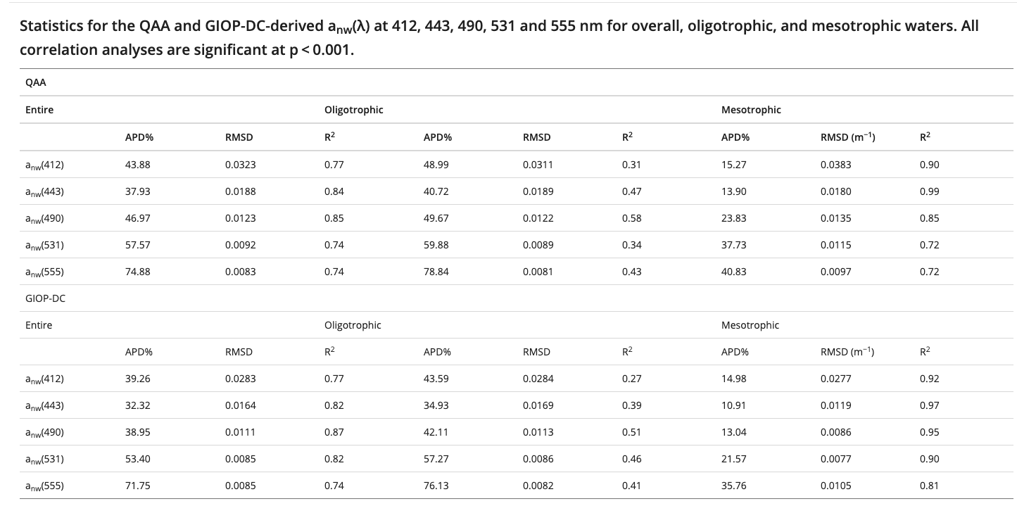
这是No-water absorption的结果

Screen Shot 0002-12-17 at 11.49.14

可看出来这俩几乎差不多

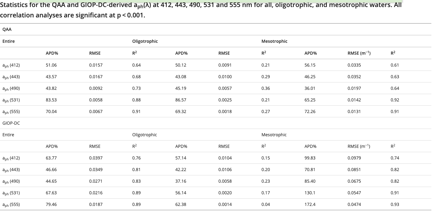
这是aph的结果

img
image-00021217115108762

GIOP表现的会比 QAA在Mesotrophic好一些

bbp

image-00021217115248284

反而是QAA

总而言之 他们发现没有特别大的区别

反而GIOP的Chla-aph关系式最好进行重新参数化